Architecture & Data Flow

Topology

Fed-MaxFuse uses a star topology: two modality nodes and one coordinating server. Each node holds exactly one modality and never sees the other's data.

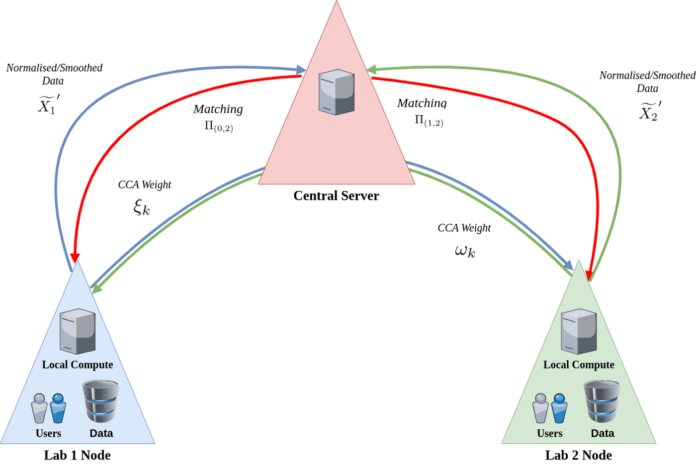
Node ↔ server communication in Fed-MaxFuse. Nodes hold raw data; the server holds none.

Simulated, not deployed

The experiments run inside a single process that simulates the federated system, with every message routed through the server component exactly as it would be over a network. This isolates algorithmic behaviour from network effects, but it means network latency, dropped messages, and node failures are untested. See Security & Privacy.

Who computes what

The split follows one rule: does this operation need both modalities at once?

Operation	Location	Why
GetSharedFeatures	Node	Uses only local data
ConstructMetaCells (Leiden)	Node	Local clustering
NearestNeighborGraph	Node	Local k-NN
FuzzySmoothing	Node	Local graph + local data
PseudoInverse	Node	Local matrix
Scores, loadings, deflation	Node	Local linear algebra
Propagate	Node	Local nearest-neighbour search
GetEmbeddingsCCA	Node	Local projection through fitted weights
LinearSumAssignment	Server	Needs the cross-modal distance matrix
Singular-vector search (SVPM)	Server	Couples both views
JoinAndAlign (propagation indices)	Server	Reconciles both nodes' index spaces
RemoveRedundantConnections	Server	Needs the joint matching
FilterOutBadMatches (β)	Server	Applied to the joined matching

Only two kinds of object ever cross the wire: normalised smoothed matrices, and latent projections/indices.

Communication protocol

The run proceeds in three phases.

1. Initialisation

NODE i:  X_i° ← GetSharedFeatures(X_i)
         X_iᵐ ← ConstructMetaCells(X_i, n_xi)
         G_Xi ← NearestNeighborGraph(X_iᵐ, k)
         X̃_i° ← FuzzySmoothing(X_i°, G_Xi, w)
         Send(X̃_i°′, to='SERVER', action='MATCHING')

SERVER:  D ← 1.0 − X̃₁°′ · (X̃₂°′)ᵀ
         {(iₖ, jₖ)} ← LinearSumAssignment(D)
         Send({(iₖ, wₖ)}, to='1');  Send({(jₖ, wₖ)}, to='2')

NODE i:  Π^{i,°} ← Receive(...)

2. Refinement loop (× T)

Each iteration runs a full FederatedCCA sub-protocol, then one matching round:

NODE i:  X_i^aligned ← X_i^cc[Π_{i−1}]
SERVER:  (X₁^cc, X₂^cc) ← FederatedCCA(X₁^aligned, X₂^aligned)   # see Iterative Federated CCA
NODE i:  X̃_i^cc ← FuzzySmoothing(X_i^cc, G_Xi, w)
         Send(X̃_i^cc′, to='SERVER', action='MATCHING')
SERVER:  ServerMatching(...)  →  Π_(i−1, 2)

3. Finalisation

Pivot filtering (local: the weights are shared, so both nodes agree), server-orchestrated embedding fit, local propagation, server-side join, a final matching round, then local embedding computation. See Final Matching & Propagation.

What crosses the wire

Object	Sent in	What it is
X̃′	init, loop, final	L2-normalised, fuzzily-smoothed feature matrix
Π	init, loop, final	Matched indices + similarity scores
ξ_k, ω_k	SVPM inner loop	Latent score vectors, length N (samples)
δ	SVPM inner loop	Scalar convergence norm

Note the dimensions. A node's active data is N × p; a latent score vector is N × 1. For the tonsil RNA node that is 10,000 floats instead of 17 million, and what is sent is already a projection, not features.

Message complexity

The dominant term is the CCA sub-protocol:

\[ \text{messages} \;\approx\; T \times C \times K \]

where T is the number of refinement iterations, C the number of CCA components, and K the maximum singular-vector power-method iterations. With T=3, C=20, K=2,000 this is the system's principal cost, not floating-point work. This is the main scalability limitation; see Security & Privacy for the discussion of decentralised alternatives.

Data layout per node

Each node needs two matrices for its modality:

Matrix	Contents	Used for
Shared (X°)	Feature-aligned columns, one-to-one with the other modality	Seed matching only
Active (X)	All features of the modality	Graphs, CCA, final embeddings

The shared matrices must have identical column counts in matching order across nodes, and each node's shared and active matrices must describe the same cells in the same row order. See Local Preprocessing.