Iterative Federated CCA

The algorithmic heart of Fed-MaxFuse, and the part that required the most work to federate.

Why not classical CCA

CCA finds linear combinations \(u = X\mathbf{a}\) and \(v = Y\mathbf{b}\) (canonical variates) that are maximally correlated:

\[ \max_{\mathbf{a},\, \mathbf{b}} \ \rho\big(u = X\mathbf{a},\; v = Y\mathbf{b}\big) \]

In practice classical CCA overfits badly when the sample size is small relative to the number of variables, producing spurious associations that do not generalise. That is precisely the single-cell regime: 10,000 cells against 20,729 features.

MaxFuse therefore uses Two-block Mode B PLS (Wold; Wegelin), which builds latent score vectors iteratively and weights indicators by predictive association. It is advantageous when indicator quality is heterogeneous, which again describes single-cell data. Fed-MaxFuse federates that method rather than textbook CCA.

This is where the federated work is

The reference implementation calls sklearn.cross_decomposition.CCA, a black box. Federating required opening it into explicit score, loading, and deflation steps so the one genuinely coupled operation could be distributed. That decomposition is the part upstream never had to write down.

The deflation loop

For each component \(c = 1 \ldots C\):

1. \(u_c,\ v_c \leftarrow \texttt{SingularVectorPowerMethod}(X^1_c,\, X^2_c)\) ← coupled
2. Node 1: \(\xi_c \leftarrow X^1_c \cdot u_c\) (scores)
3. Node 1: \(\gamma_c^\top \leftarrow \xi_c(\xi_c^\top \xi_c)^{-1}\xi_c^\top X^1_c\) (loadings)
4. Node 1: \(\hat{X^1}_c \leftarrow \xi_c \cdot \gamma_c^\top\), then \(X^1_{c+1} \leftarrow X^1_c - \hat{X^1}_c\) (deflation)
5. Node 2 mirrors with \(\omega_c,\ \delta_c,\ X^2\)

Steps 2–5 are entirely local. Only step 1 requires communication. After \(C\) components, the transformation matrices are assembled as \(U\Gamma^\top\) and \(V\Delta^\top\).

That asymmetry, one coupled step out of five, is the seam that makes the whole thing federable. Look for the same seam in any iterative component-extraction method.

The federated singular-vector power method

The coupled step approximates the leading singular vectors of the cross-correlation matrix \(\mathbf{C} = (X^1_c)^\top X^2_c\), which neither node can form, since it spans both feature spaces.

The key insight: the power iteration only ever needs the other side's latent score vector, an \(N\)-vector with one entry per sample, not the features.

Input (nodes):  residuals X^i_c ∈ ℝ^{N×n_i}
Input (server): max iterations K, tolerance ε, interpolation weight w

# NODE 1&2 — local initialisation
ξ₁ or ω₁   ← NoiseInterpolation(X^i_c[:,0], w)
X_c^{i,†}  ← PseudoInverse(X^i_c)             # (XᵀX)⁻¹Xᵀ, computed ONCE per component

# SERVER-driven loop
k ← 1;  δ ← ∞
while δ > ε and k < K:
    Send(ξ_k, to='2', via='SERVER')            # NODE 1
    Send(ω_k, to='1', via='SERVER')            # NODE 2

    Receive(ω_k or ξ_k)                        # NODE 1&2
    l_k                ← ω_k or ξ_k
    u_k or v_k         ← X_c^{i,†} · l_k (l_kᵀ l_k)⁻¹
    u_k or v_k         ← Normalize(u_k or v_k)
    ω_{k+1} or ξ_{k+1} ← X_c^i · (u_k or v_k)

    δ ← ‖u_k − u_{k−1}‖                        # NODE 1 only
    Send(δ, to='SERVER')
    k ← k + 1

Three implementation requirements:

• Mode B needs the Moore–Penrose pseudo-inverse \(X^\dagger = (X^\top X)^{-1}X^\top\), computed locally, once per component, not inside the iteration.
• Normalize every iteration or the power method loses convergence stability. This is a requirement, not cosmetics.
• A sign convention forces the largest-magnitude element of \(u_c\) positive after a possible flip, so components are deterministic in sign across nodes.

Noise interpolation at initialisation

The textbook power method initialises latent scores from a real data column, \(X_c^i[:,0]\), which would mean sharing a column of real data. Fed-MaxFuse interpolates with Gaussian noise instead:

\[ \texttt{NoiseInterpolation}(v, w) = (1-w)\cdot v \;+\; w \cdot \mathcal{N}(0,1)^n, \qquad w \in (0.0,\, 1.0] \]

\(w = 0.0\) is explicitly undesirable: it means a real data column is shared.

The empirical result is that this privacy is essentially free:

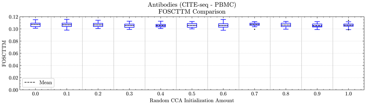
FOSCTTM across noise-interpolation weights \(w \in [0,1]\). The curve is flat.

Integration quality is remarkably stable across the whole range, with the lowest median FOSCTTM at around \(w = 0.6\), a slight improvement, plausibly because moderate stochasticity helps the singular-vector updates escape poor local optima. FOSKNN is similarly flat.

Recommended setting

Use \(w \approx 0.6\). There is no accuracy argument for a low \(w\), and \(w = 0\) leaks a data column for zero measured benefit.

Cost

Per refinement round: \(C\) components, each needing up to \(K\) power-method iterations, each of which exchanges two \(N\)-vectors plus one scalar. Over \(T\) outer loops that is

\[ T \times C \times K \]

round trips in the worst case, the dominant cost of the entire system. With \(T\)=3, \(C\)=20 and \(K\)=2,000 this, not arithmetic, is what limits scaling.

Configuration

"refinement_loop": {
  "cca": {
    "randomness": 0.6,
    "components": 20,
    "max_loop_iterations": 2000,
    "bad_filter_wt": 0.0
  },
  "loop_iterations": 3
}

Key	Symbol	Meaning
components	\(C\)	Shared components
max_loop_iterations	\(K\)	SVPM iteration cap
randomness	\(w\)	Noise interpolation weight
loop_iterations	\(T\)	Outer refinement rounds

The CCAType enum selects the implementation: sklearn (centralized reference), pseudo, plswtb (Two-block Mode B PLS), and plswtb_rand_init (with noise interpolation).