Federated Matching Stage
How two nodes agree on which cells correspond, without either seeing the other's data.
The centralized problem
MaxFuse turns matching into a linear sum assignment problem. Given a cross-modal distance matrix \(\mathbf{D}\), find the binary assignment \(M\) minimising total distance:
solved exactly by the Jonker–Volgenant algorithm. The distance is one minus Pearson correlation, \(\mathbf{D} = 1 - \rho\), which converts similarity maximisation into distance minimisation.
Why it federates
Pearson correlation factorises. Write the mean-centred, L2-normalised matrix as
Then
which is a plain dot product. So each node can do its own centring and normalising locally, and the server needs only
This is mathematically identical to the centralized computation. No approximation is involved.
The server matching procedure
Input:  normalised, smoothed X₁′ ∈ ℝ^{N₁×p₁},  X₂′ ∈ ℝ^{N₂×p₂}
Output: {(iₖ, wₖ)} to node 1,  {(jₖ, wₖ)} to node 2

Receive(X₁′, from='1', action='MATCHING')
Receive(X₂′, from='2', action='MATCHING')

D          ← 1.0 − X₁′ · (X₂′)ᵀ            # inverse of Pearson
{(iₖ,jₖ)}  ← LinearSumAssignment(D)
{wₖ}       ← D[{(iₖ,jₖ)}]

Send({(iₖ, wₖ)}, to='1', action='MATCHING')
Send({(jₖ, wₖ)}, to='2', action='MATCHING')
Three properties worth noting:
- The server is stateless: it holds nothing between calls.
- It never inverts a matrix and never learns feature semantics.
- It is reused at three points in the pipeline: initial matching, each refinement iteration, and the final propagation matching.
What each party learns
| Party | Learns | Does not learn |
|---|---|---|
| Node 1 | Its own indices + match scores | Which of node 2's cells it matched |
| Node 2 | Its own indices + match scores | Which of node 1's cells it matched |
| Server | The full index correspondence; normalised smoothed matrices | Raw feature values |
This is the Split-Π convention: indices private, weights shared. Sharing the weights is what lets both nodes apply the same pivot filter independently, with no extra round trip.
Initial matching quality
The seed matching is computed from the shared features only: 177 columns for Antibodies, 32 for Tonsils. It is correspondingly noisy, and that is expected. Its job is to be better than random so the refinement loop has something to amplify.
The experiments bear this out sharply:
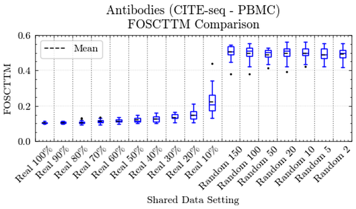
FOSCTTM under varying shared-feature selection. Real features (left) versus randomly chosen ones (right).
- Using 60–80% of true shared features gives performance near the full-set optimum. The method is robust to incomplete correspondence.
- Substituting randomly selected features severely degrades integration: much worse FOSKNN, much higher FOSCTTM.
The distinction matters: MaxFuse tolerates losing correspondences, but not replacing them with noise. A random seed gives the bootstrap nothing to amplify. Curate the shared feature set, or do not run.
Anti-patterns
- Sending raw or merely mean-centred features. The smoothing step is what degrades individual-cell recoverability. Skipping it for speed defeats the privacy design.
- Letting a node compute the full matching. It would need the other modality's matrix.
- Assuming index-only exchange is automatically safe. Indices can hint at sample relationships if improperly aggregated.